Global and Local Measures of Spatial Association - sfdep Methods

1. Overview

2. Getting Started

2.1. Installing and Loading the R Packages

Four R Packages will be used for this in-class exercise, they are: sf, sfdep, tmap, tidyverse, knitr.

pacman::p_load(sf, sfdep, tmap, tidyverse, knitr)

3. The Data

For the purpose of this in-class, exercise, the Hunan data sets will be used. There are two data sets in this use case, they are:

• Hunan, a geospatial data set in ESRI shapefile format, and

• Hunan_2012, an attribute data set in csv format.

3.1. Importing Geospatial Data

hunan <- st_read(dsn = "data/geospatial", 
                     layer = "Hunan")

Reading layer `Hunan' from data source 
  `D:\scwsu\ISSS624\In-class Ex\In-class_Ex2\data\geospatial' 
  using driver `ESRI Shapefile'
Simple feature collection with 88 features and 7 fields
Geometry type: POLYGON
Dimension:     XY
Bounding box:  xmin: 108.7831 ymin: 24.6342 xmax: 114.2544 ymax: 30.12812
Geodetic CRS:  WGS 84

3.2. Importing Attribute Table

hunan2012 <- read_csv("data/aspatial/Hunan_2012.csv")

3.3. Combining Both Data Frame by Using Left Join

hunan_GDPPC <- left_join(hunan,hunan2012) %>%      
  select(1:4, 7, 15)

Important

In order to retain the geospatial properties, the left data frame must be sf data.frame (i.e. hunan).

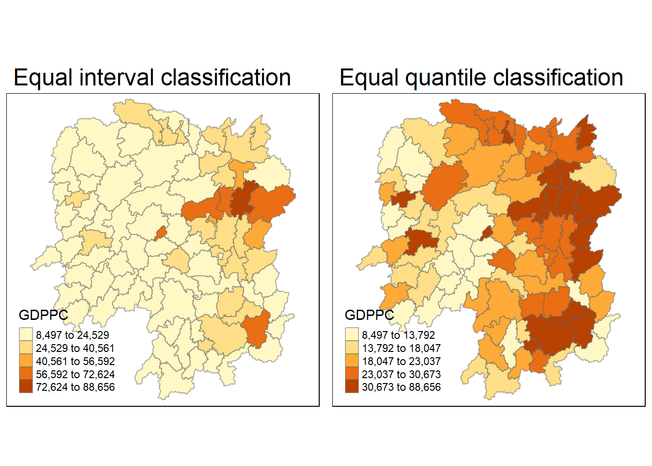
3.4. Plotting a Choropleth Map

equal <- tm_shape(hunan_GDPPC) +
  tm_fill("GDPPC",
          n = 5,
          style = "equal") +
  tm_borders(alpha = 0.5) +
  tm_layout(main.title = "Equal interval classification")

quantile <- tm_shape(hunan_GDPPC) +
  tm_fill("GDPPC",
          n = 5,
          style = "quantile") +
  tm_borders(alpha = 0.5) +
  tm_layout(main.title = "Equal quantile classification")

tmap_arrange(equal, 
             quantile, 
             asp=1, 
             ncol=2)

4. Deriving Contiguity Weights

#wm_q <- poly2nb(hunan, 
                #queen=TRUE)
#summary(wm_q)

4.1. Deriving Contiguity Weights: Queen’s Method

wm_q<- hunan_GDPPC %>%
  mutate(nb = st_contiguity(geometry),
         wt = st_weights(nb,
                         style = "W"),
         .before = 1)

Notice that st_weights() provides tree arguments, they are:

• nb: A neighbor list object as created by st_neighbors().

• style: Default “W” for row standardized weights. The style argument can take values such as “W,” “B,” “C,” “U,” “minmax,” and “S.” “B” represents basic binary coding, “W” stands for row-standardized (sums over all links to n), “C” denotes globally standardized (sums over all links to n), “U” is equal to “C” divided by the number of neighbors (sums over all links to unity), and “S” corresponds to the variance-stabilizing coding scheme proposed by Tiefelsdorf et al. 1999, p. 167-168 (sums over all links to n).

5. Computing Local Moran’s I

lisa <- wm_q %>%
  mutate(local_moran = local_moran(
    GDPPC, nb, wt, nsim = 99),
    .before = 1) %>%
  unnest(local_moran)

The output of local_moran() is a sf data frame containing the columns ii, eli, var_ii, z_ii, p_ii, p_ii_sim, and p_folded_sim.