Spatial Econometrics Interaction Modelling

Author

Su Sandi Cho Win

Published

December 16, 2023

Modified

December 16, 2023

devtools::install_github("LukeCe/spflow")

pacman::p_load(tmap, sf, spdep, sp, Matrix, spflow, reshape2, knitr, tidyverse)

Data Preparation

Before we can calibrate Spatial Econometric Interaction models by using spflow package, three data sets are required. They are:

a spatial weights,
a tibble data.frame consists of the origins, destination, flows and distances between the origins and destination, and
a tibble data.frame consists of the explanatory variables.

Building the Geographical Area

For the purpose of this study, URA Master Planning 2019 Planning Subzone GIS data will be used.

In the code chunk below, MPS-2019 shapefile will be imported into R environment as a sf tibble data.frame called mpsz.

# mpsz <- st_read(dsn = "data/geospatial", layer = "MPSZ-2019") %>%
#   st_transform(crs = 3414)

In this study, our analysis will be focused on planning subzone with bus stop. In view of this, the code chunk below will be used to

# mpsz$'BUSSTOP_COUNT' <- lengths(
#   st_intersects(mpsz, busstop)
# )

# mpsz_busstop <- mpsz %>%
#   filter(BUSSTOP_COUNT > 0)
# mpsz_busstop

Preparing Spatial Weights

# centroids <- suppressWarnings({
#   st_point_on_surface(st_geometry(mpsz_busstop))
# })
# 
# mpsz_nb <- list(
#   "by_contiguity" = poly2nb(mpsz_busstop),
#   "by_distance" = dnearneigh(centroids, d1 = 0, d2 = 5000),
#   "by_knn" = knn2nb(knearneigh(centroids, 3))
# )

# mpsz_nb

#write_rds(mpsz_nb, "data/rds/mpsz_nb.rds")

# odbus6_9 <- read_rds("data/rds/odbus6_9.rds")

# busstop_mpsz <- st_intersection(busstop, mpsz) %>%
#   select(BUS_STOP_N, SUBZONE_C) %>%
#   st_drop_geometry()

# od_data <- left_join(odbus6_9 , busstop_mpsz,
#                      by = c("ORIGIN_PT_CODE" = "BUS_STOP_N")) %>%
#   rename(ORIGIN_BS = ORIGIN_PT_CODE,
#          ORIGIN_SZ = SUBZONE_C,
#          DESTIN_BS = DESTINATION_PT_CODE)

# duplicate <- od_data %>%
#   group_by_all() %>%
#   filter(n() > 1) %>%
#   ungroup()

# od_data <- unique(od_data)

# od_data <- left_join(od_data , busstop_mpsz,
#                      by = c("DESTIN_BS" = "BUS_STOP_N"))

# duplicate <- od_data %>%
#   group_by_all() %>%
#   filter(n() > 1) %>%
#   ungroup()

# od_data <- unique(od_data)

# od_data <- od_data %>%
#   rename(DESTIN_SZ = SUBZONE_C) %>%
#   drop_na() %>%
#   group_by(ORIGIN_SZ, DESTIN_SZ) %>%
#   summarise(MORNING_PEAK = sum(TRIPS))

# mpsz_sp <- as(mpsz, "Spatial")
# mpsz_sp

# dist <- spDists(mpsz_sp, 
#                 longlat = FALSE)
# head(dist, n=c(10, 10))

# sz_names <- mpsz$SUBZONE_C

# colnames(dist) <- paste0(sz_names)
# rownames(dist) <- paste0(sz_names)

# distPair <- melt(dist) %>%
#   rename(dist = value)
# head(distPair, 10)

# distPair %>%
#   filter(dist > 0) %>%
#   summary()

# distPair$dist <- ifelse(distPair$dist == 0,
#                         50, distPair$dist)

# distPair %>%
#   summary()

# distPair <- distPair %>%
#   rename(orig = Var1,
#          dest = Var2)

# write_rds(distPair, "data/rds/distPair.rds")

# mpsz_var

# write_rds(mpsz_var, "data/rds/mpsz_var.rds")

mpsz_nb <- read_rds("data/rds/mpsz_nb.rds")
mpsz_flow <- read_rds("data/rds/mpsz_flow.rds")
mpsz_var <- read_rds("data/rds/mpsz_var.rds")

Creating `spflow_network-class` object

spflow_network-class is an S4 class that contains all information on a spatial network which is composed by a set of nodes that are linked by some neighborhood relation. It can be created by using https://lukece.github.io/spflow/reference/spflow_network.html of spflow package.

For our model, we choose the contiguity based neighborhood structure.

mpsz_net <- spflow_network(
  id_net = "sg",
  node_neighborhood = 
    nb2mat(mpsz_nb$by_contiguity),
  node_data = mpsz_var,
  node_key_column = "SZ_CODE")

mpsz_net

Spatial network nodes with id: sg
--------------------------------------------------
Number of nodes: 313
Average number of links per node: 6.077
Density of the neighborhood matrix: 1.94% (non-zero connections)

Data on nodes:
                SZ_NAME SZ_CODE BUSSTOP_COUNT AGE7_12 AGE13_24 AGE25_64
1      INSTITUTION HILL  RVSZ05             2     330      360     2260
2        ROBERTSON QUAY  SRSZ01            10     320      350     2200
3          FORT CANNING  MUSZ02             6       0       10       30
4      MARINA EAST (MP)  MPSZ05             2       0        0        0
5               SENTOSA  SISZ01             1     200      260     1440
6        CITY TERMINALS  BMSZ17            10       0        0        0
---                 ---     ---           ---     ---      ---      ---
308            NEE SOON  YSSZ07            12      90      140      590
309       UPPER THOMSON  BSSZ01            47    1590     3660    15980
310          SHANGRI-LA  AMSZ05            12     810     1920     9650
311          TOWNSVILLE  AMSZ04             9     980     2000    11320
312           MARYMOUNT  BSSZ02            25    1610     4060    16860
313 TUAS VIEW EXTENSION  TSSZ06            11       0        0        0
    SCHOOL_COUNT BUSINESS_COUNT RETAILS_COUNT FINSERV_COUNT ENTERTN_COUNT
1              1              6            26             3             0
2              0              4           207            18             6
3              0              7            17             0             3
4              0              0             0             0             0
5              0              1            84            29             2
6              0             11            14             4             0
---          ---            ---           ---           ---           ---
308            0              0             7             0             0
309            3             21           305            30             0
310            3              0            53             9             0
311            1              0            83            11             0
312            3             19           135             8             0
313            0             53             3             1             0
    FB_COUNT LR_COUNT COORD_X COORD_Y
1          4        3  103.84    1.29
2         38       11  103.84    1.29
3          4        7  103.85    1.29
4          0        0  103.88    1.29
5         38       20  103.83    1.25
6         15        0  103.85    1.26
---      ---      ---     ---     ---
308        0        0  103.81     1.4
309        5       11  103.83    1.36
310        0        0  103.84    1.37
311        1        1  103.85    1.36
312        3       11  103.84    1.35
313        0        0  103.61    1.26

mpsz_net_pairs <- spflow_network_pair(
  id_orig_net = "sg",
  id_dest_net = "sg",
  pair_data = mpsz_flow,
  orig_key_column = "ORIGIN_SZ",
  dest_key_column = "DESTIN_SZ")

mpsz_net_pairs

Spatial network pair with id: sg_sg
--------------------------------------------------
Origin network id: sg (with 313 nodes)
Destination network id: sg (with 313 nodes)
Number of pairs: 97969
Completeness of pairs: 100.00% (97969/97969)

Data on node-pairs:
      DESTIN_SZ ORIGIN_SZ DISTANCE TRIPS
1        RVSZ05    RVSZ05        0    67
314      SRSZ01    RVSZ05   305.74   251
627      MUSZ02    RVSZ05   951.83     0
940      MPSZ05    RVSZ05  5254.07     0
1253     SISZ01    RVSZ05     4975     0
1566     BMSZ17    RVSZ05  3176.16     0
---         ---       ---      ---   ---
96404    YSSZ07    TSSZ06 26972.97     0
96717    BSSZ01    TSSZ06 25582.48     0
97030    AMSZ05    TSSZ06 26714.79     0
97343    AMSZ04    TSSZ06 27572.74     0
97656    BSSZ02    TSSZ06  26681.7     0
97969    TSSZ06    TSSZ06        0   270

mpsz_multi_net <- spflow_network_multi(mpsz_net, mpsz_net_pairs)
mpsz_multi_net

Collection of spatial network nodes and pairs
--------------------------------------------------
Contains 1 spatial network nodes  
    With id :  sg
Contains 1 spatial network pairs  
    With id :  sg_sg

Availability of origin-destination pair information:

 ID_ORIG_NET ID_DEST_NET ID_NET_PAIR COMPLETENESS     C_PAIRS  C_ORIG  C_DEST
          sg          sg       sg_sg      100.00% 97969/97969 313/313 313/313

cor_formula <- log(1 + TRIPS) ~
  BUSSTOP_COUNT +
  AGE7_12 +
  AGE13_24 +
  AGE25_64 +
  SCHOOL_COUNT +
  BUSINESS_COUNT +
  RETAILS_COUNT +
  FINSERV_COUNT +
  P_(log(DISTANCE + 1)) #P_ is only applicable if you are using distance or cost (impedance)

cor_mat <- pair_cor(
  mpsz_multi_net,
  spflow_formula = cor_formula,
  add_lags_x = FALSE) #lag is the distance neighborhood. We are including in this case.

colnames(cor_mat) <- paste0(
  substr(
    colnames(cor_mat),1,3),"...")

cor_image(cor_mat)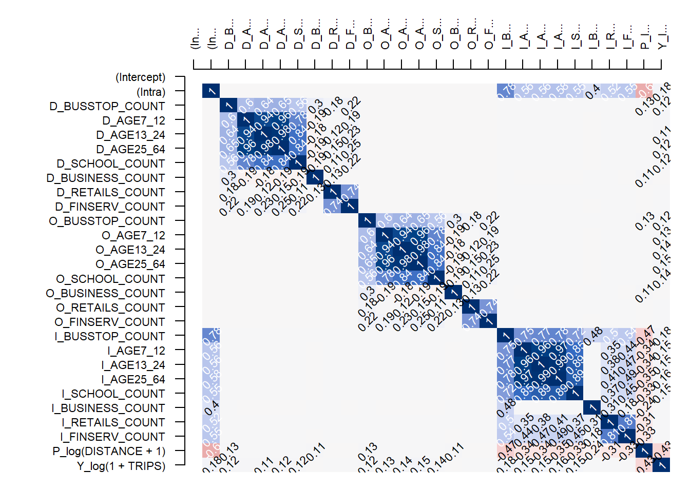

base_model <- spflow(
  spflow_formula =  log(1 + TRIPS) ~
    O_(BUSSTOP_COUNT +
         AGE25_64) +
    D_(SCHOOL_COUNT +
         BUSINESS_COUNT +
         RETAILS_COUNT +
         FINSERV_COUNT) +
    P_(log(DISTANCE + 1)),
  spflow_networks = mpsz_multi_net)

base_model

--------------------------------------------------
Spatial interaction model estimated by: MLE  
Spatial correlation structure: SDM (model_9)
Dependent variable: log(1 + TRIPS)

--------------------------------------------------
Coefficients:
                          est     sd   t.stat  p.val
rho_d                   0.680  0.004  192.553  0.000
rho_o                   0.678  0.004  187.734  0.000
rho_w                  -0.396  0.006  -65.592  0.000
(Intercept)             0.410  0.065    6.267  0.000
(Intra)                 1.312  0.081   16.262  0.000
D_SCHOOL_COUNT          0.017  0.002    7.885  0.000
D_SCHOOL_COUNT.lag1     0.002  0.004    0.552  0.581
D_BUSINESS_COUNT        0.000  0.000    3.015  0.003
D_BUSINESS_COUNT.lag1   0.000  0.000   -0.249  0.804
D_RETAILS_COUNT         0.000  0.000   -0.306  0.759
D_RETAILS_COUNT.lag1    0.000  0.000    0.152  0.880
D_FINSERV_COUNT         0.002  0.000    6.787  0.000
D_FINSERV_COUNT.lag1   -0.002  0.001   -3.767  0.000
O_BUSSTOP_COUNT         0.002  0.000    6.807  0.000
O_BUSSTOP_COUNT.lag1   -0.001  0.000   -2.364  0.018
O_AGE25_64              0.000  0.000    7.336  0.000
O_AGE25_64.lag1         0.000  0.000   -2.797  0.005
P_log(DISTANCE + 1)    -0.050  0.007   -6.794  0.000

--------------------------------------------------
R2_corr: 0.6942948  
Observations: 97969  
Model coherence: Validated

old_par <- par(mfrow = c(1, 3),
               mar = c(2,2,2,2))
spflow_moran_plots((base_model))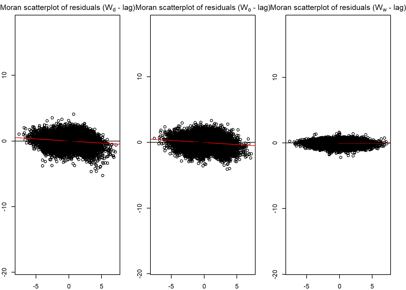

par(old_par)

corr_residual <- pair_cor(base_model)
colnames(corr_residual) <- substr(colnames(corr_residual), 1, 3)
cor_image(corr_residual)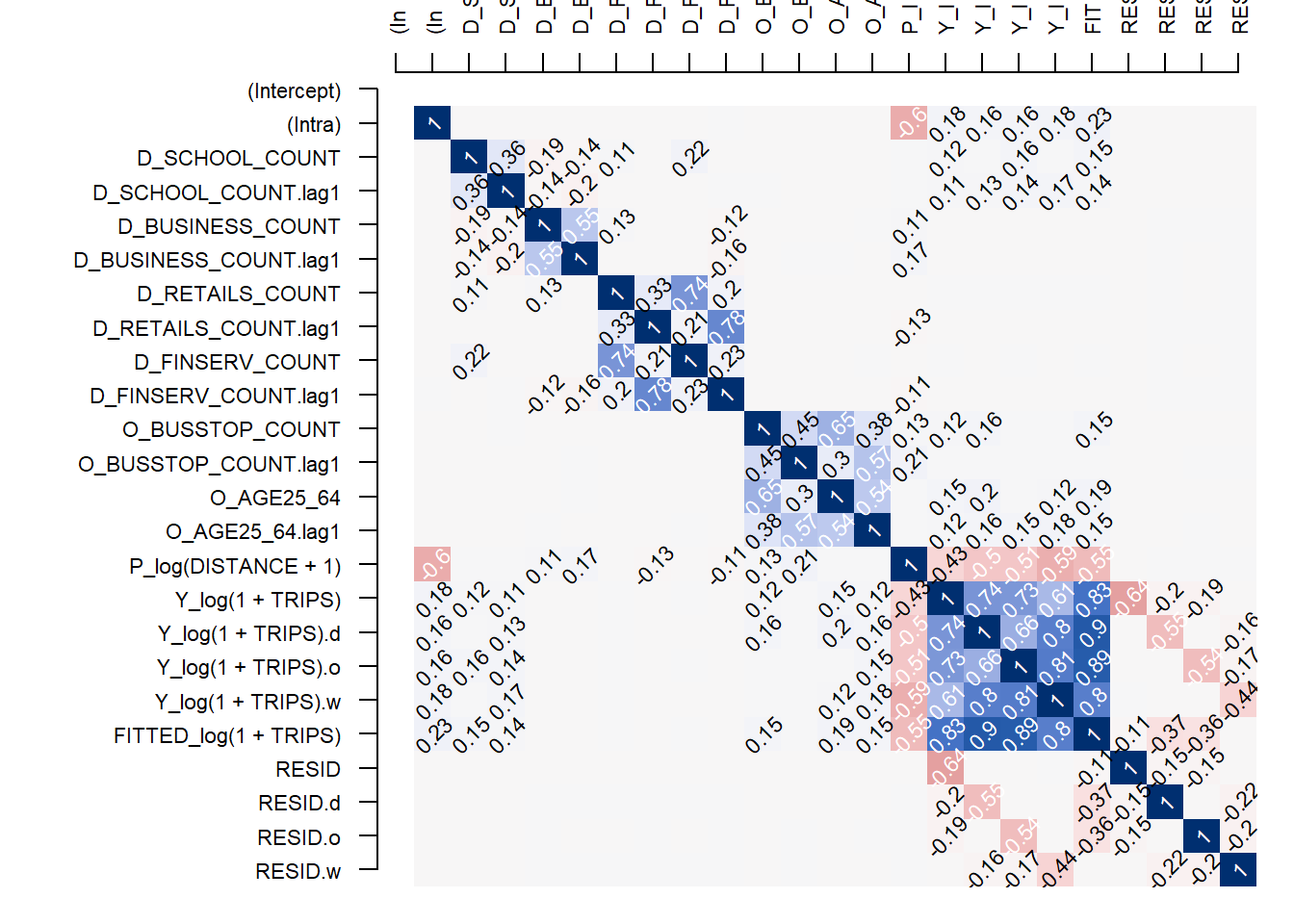

spflow_formula <- log(1 + TRIPS) ~
    O_(BUSSTOP_COUNT +
         AGE25_64) +
    D_(SCHOOL_COUNT +
         BUSINESS_COUNT +
         RETAILS_COUNT +
         FINSERV_COUNT) +
    P_(log(DISTANCE + 1))


model_control <- spflow_control(
  estimation_method = "mle",
  model = "model_1")

mle_model1 <- spflow(
  spflow_formula,
  spflow_networks = mpsz_multi_net,
  estimation_control = model_control)

mle_model1

--------------------------------------------------
Spatial interaction model estimated by: OLS  
Spatial correlation structure: SLX (model_1)
Dependent variable: log(1 + TRIPS)

--------------------------------------------------
Coefficients:
                          est     sd    t.stat  p.val
(Intercept)            11.384  0.069   164.255  0.000
(Intra)                -6.006  0.112   -53.393  0.000
D_SCHOOL_COUNT          0.093  0.003    28.599  0.000
D_SCHOOL_COUNT.lag1     0.255  0.006    44.905  0.000
D_BUSINESS_COUNT        0.001  0.000    10.036  0.000
D_BUSINESS_COUNT.lag1   0.003  0.000    18.274  0.000
D_RETAILS_COUNT         0.000  0.000    -1.940  0.052
D_RETAILS_COUNT.lag1    0.000  0.000    -2.581  0.010
D_FINSERV_COUNT         0.005  0.000    10.979  0.000
D_FINSERV_COUNT.lag1   -0.016  0.001   -17.134  0.000
O_BUSSTOP_COUNT         0.014  0.001    25.865  0.000
O_BUSSTOP_COUNT.lag1    0.015  0.001    21.728  0.000
O_AGE25_64              0.000  0.000    14.479  0.000
O_AGE25_64.lag1         0.000  0.000    14.452  0.000
P_log(DISTANCE + 1)    -1.281  0.008  -165.327  0.000

--------------------------------------------------
R2_corr: 0.2831458  
Observations: 97969  
Model coherence: Validated

Data Preparation

Building the Geographical Area

Preparing Spatial Weights

Creating spflow_network-class object

Creating `spflow_network-class` object