Urban Mobility Analysis

1. Overview

Urban Mobility Analysis by using passenger volume by origin-destination bus stops.

2. Getting Started

The code chunk below loads the following packages:

• tmap: for thematic mapping
• sf: for geospatial data handling
• tidyverse: for non-spatial data handling

pacman::p_load(sf, tmap, tidyverse, knitr)

The data used for this analysis includes:

• Subzone Boundary Data from the Master Plan 2019 (last updated Dec 2019) from data.gov.sg.

• Bus Stop Location Data (last updated Jul 2023) obtained from LTADataMall.

• Passenger Volume Data for Aug-Oct 2023, focusing on origin and destination bus stops, also retrieved from LTADataMall.

3. Preparing Flow Data

3.1. Importing Passenger Volume by Origin-Destination Bus Stops

Firstly, we will import the Passenger Volume by Origin-Destination Bus Stops data set download from LTADataMall by using `read_csv()` of readr package and name the dataframe as `odbus`.

odbus <- read_csv("data/aspatial/origin_destination_bus_202308.csv")

To treat the numeric variables `ORIGIN_PT_CODE` and `DESTINATION_PT_CODE` as categorical grouping variables in R, they should be converted to factors. This transformation allows R to recognize and work with them as categorical variables.

odbus$ORIGIN_PT_CODE <- as.factor(odbus$ORIGIN_PT_CODE)
odbus$DESTINATION_PT_CODE <- as.factor(odbus$DESTINATION_PT_CODE) 

origin7_9 <- odbus %>%
  filter(DAY_TYPE == "WEEKDAY") %>%
  filter(TIME_PER_HOUR >= 7 &
           TIME_PER_HOUR <= 9) %>%
  group_by(ORIGIN_PT_CODE) %>%
  summarise(TRIPS = sum(TOTAL_TRIPS))

write_rds(origin7_9, "data/rds/origin7_9.rds")

origin7_9 <- read_rds("data/rds/origin7_9.rds")

3.2. Extracting Commuting Flow Data

The following code chunk extracts data related to commuting patterns on weekdays during the busy morning rush hours (7 am, 8 am, and 9 am).

3.3. Importing Geospatial Data

The following code chunk uses `st_read()` function from the sf package to import `BusStop` shapefile into R dataframe named `BusStop`. It is configured with the svy21 projected coordinate system, with a `crs` setting of 3414.

busstop <- st_read(dsn = "data/geospatial",
                   layer = "BusStop") %>%
  st_transform(crs = 3414)

Reading layer `BusStop' from data source 
  `D:\scwsu\ISSS624\In-class Ex\In-class_Ex1\data\geospatial' 
  using driver `ESRI Shapefile'
Simple feature collection with 5161 features and 3 fields
Geometry type: POINT
Dimension:     XY
Bounding box:  xmin: 3970.122 ymin: 26482.1 xmax: 48284.56 ymax: 52983.82
Projected CRS: SVY21

3.4. Importing Planning Subzone Data

The following code chunk uses `st_read()` function from the sf package to import `MPSZ-2019` shapefile into R dataframe named `mpsz`. To enable the combined use of `mpsz` with `BusStop`, `mpsz` is configured with the svy21 projected coordinate system, with a `crs` setting of 3414.

mpsz <- st_read(dsn = "data/geospatial",
                   layer = "MPSZ-2019") %>%
  st_transform(crs = 3414)

Reading layer `MPSZ-2019' from data source 
  `D:\scwsu\ISSS624\In-class Ex\In-class_Ex1\data\geospatial' 
  using driver `ESRI Shapefile'
Simple feature collection with 332 features and 6 fields
Geometry type: MULTIPOLYGON
Dimension:     XY
Bounding box:  xmin: 103.6057 ymin: 1.158699 xmax: 104.0885 ymax: 1.470775
Geodetic CRS:  WGS 84

3.4. Data Wrangling - Geospatial Data

busstop_mpsz <- st_intersection(busstop, mpsz) %>%
  select(BUS_STOP_N, SUBZONE_C) %>%
  st_drop_geometry()

write_rds(busstop_mpsz, "data/rds/busstop_mpsz.csv")  

origin_SZ <- left_join(origin7_9 , busstop_mpsz,
            by = c("ORIGIN_PT_CODE" = "BUS_STOP_N")) %>%
  rename(ORIGIN_BS = ORIGIN_PT_CODE,
         ORIGIN_SZ = SUBZONE_C) %>%
  group_by(ORIGIN_SZ) %>%
  summarise(TOT_TRIPS = sum(TRIPS))

duplicate <- origin_SZ %>%
  group_by_all() %>%
  filter(n()>1) %>%
  ungroup()

origin_data <- unique(origin_SZ)

origintrip_SZ <- left_join(mpsz, 
                           origin_SZ,
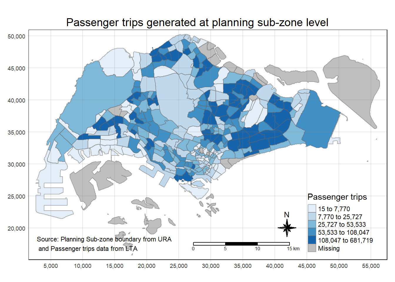
                           by = c("SUBZONE_C" = "ORIGIN_SZ"))

tm_shape(origintrip_SZ)+
  tm_fill("TOT_TRIPS", 
          style = "quantile", 
          palette = "Blues",
          title = "Passenger trips") +
  tm_layout(main.title = "Passenger trips generated at planning sub-zone level",
            main.title.position = "center",
            main.title.size = 1.2,
            legend.height = 0.45, 
            legend.width = 0.35,
            frame = TRUE) +
  tm_borders(alpha = 0.5) +
  tm_compass(type="8star", size = 2) +
  tm_scale_bar() +
  tm_grid(alpha =0.2) +
  tm_credits("Source: Planning Sub-zone boundary from URA\n and Passenger trips data from LTA", 
             position = c("left", "bottom"))